I. OVERVIEW: THE BIG IDEA

This project proposal aims to use structural equation models to gain a deeper understanding of the Reno/Sparks community in terms of city growth. Using structural equation models will allow for a richer study of multivariate relationships, filling in the gaps where traditional linear and multiple regression fail to account for.
Namely, relationships in this model will be allowed to be interdependent with one another – covariance and error terms will be isolated and better explained, and complex relationships will be better addressed.
TOPIC: UNDERSTANDING CITY GROWTH:

How does building growth vary through the city?
Many factors may come to mind, and that’s most definitely correct. The beauty (and fun) of learning structural equation models is that we can test all of these variables – having a hunch about something can be accurately validated.
II. LITERATURE REVIEW
1.) Migration and Residential Mobility: Macro and Micro Approaches
– by Martin Cadwaller, 1992.
This book used structural equation models to explain very similar situations to the model proposed in this study.
A key theme from the book was:
a.) the idea of “mobility“, or residential mobility. Residential mobility shapes the growth of all cities, as “20% of the U.S. population changes residence every year” (Cadwaller 153).
2.) Exploring the connections among job accessibility, employment, income, and auto ownership using structural equation modeling
– by Shengyi Gao, Patricia L. Mokhtarian & Robert A. Johnston, 2006.
This professional journal article came from the 2008 Annals of Regional Science Journal, and uses a structural equation model to better describe social, housing, and economic relationships between workers in Sacramento, CA. Crucial to my own research proposal, this paper validates the use of census-tract level U.S. Census data with structural equation modelling.
A few key points from the article are that:
a.) “to a household, choosing residential location is choosing a consumption bundle. On the one hand the willingness to pay for the bundle is subject to constraints on income, transportation availability, and commute distance allocation between the household members if a household has more than one worker” (Gao et al., 342).
b.) the basic notion that standard OLS regression would not serves as a proper means to analyze this study, as the error term in one independent variable is not independent of the other variable(s) (Gao et al., 342).
c.) “land use patterns determine locations of jobs and residences” (Gao et al., 344).
3.) Order without Design: How Markets Shape Cities
– by Alain Bertaud, 2018.
This book served mainly as a conceptual guide relating to cities and the design of cities. The principal argument states that in the majority of cases, a blind, dumb, and careless hand of ‘economic markets’ designs the landscape we live in for us. In other words, city design is rarely based on higher-order themes – economic markets dictate what our cities look like.
III. HYPOTHESIZED MODEL
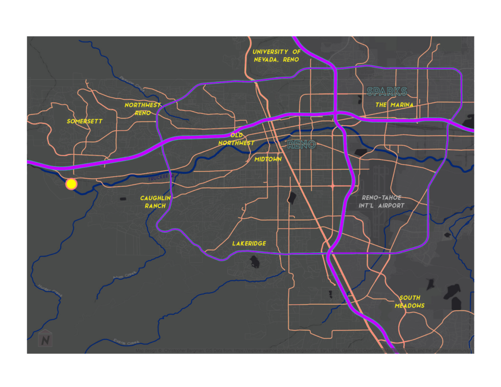
This project idea is defended and supported by other successful studies using U.S. Census data to assess multivariate trends at the city-level. Moving deeper, this study will also explore spatial location as an indicator for trends in census data and building permits.
Core Concept of Hypothesized Model:
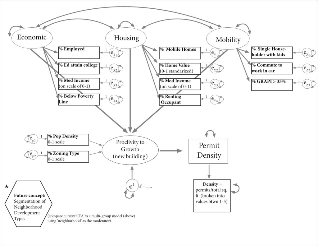
‘Proclivity to growth’ is the key concept that will be tested in this model.
Can proclivity to growth be modeled by U.S. Census data and can it be used to help describe/explain/predict the density of building permit sites in the Reno-Sparks community (building permits approved and contingent between 2020-2022)?
Justified?
This hypothesized model has yet to be justified by an experiment.
Complexity?
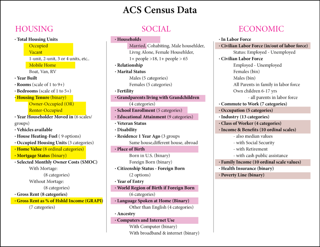
The American Community Survey (Economic, Social, and Housing) combines contain hundreds of total variates. For the sake of parsimony and optimal CFA modeling, only 12 manifest variables were chosen from the U.S. Census. The remaining 2 manifest variables were derived from zoning types and building permit density.
Identification?
The model is over-identified: with 14 manifest variables, the observations (p)= v * (v+1/2) = 105
The total number of parameters (q) (variance paths + coefficient paths) = 53, so degrees of freedom = (p-q) = 105 – 53 = 52. This means that each variable in the model has a least 1 solution.
Hypothesized Model:
IV. PLANNED METHODS
VARIABLES TO INTERPRET:
- 1.) American Community Survey (U.S. Census)
- Economic Characteristics
- Housing Characteristics
- Social Characteristics
- 2.) Washoe County Building Permits
- Permits requested and approved, 2020-2022
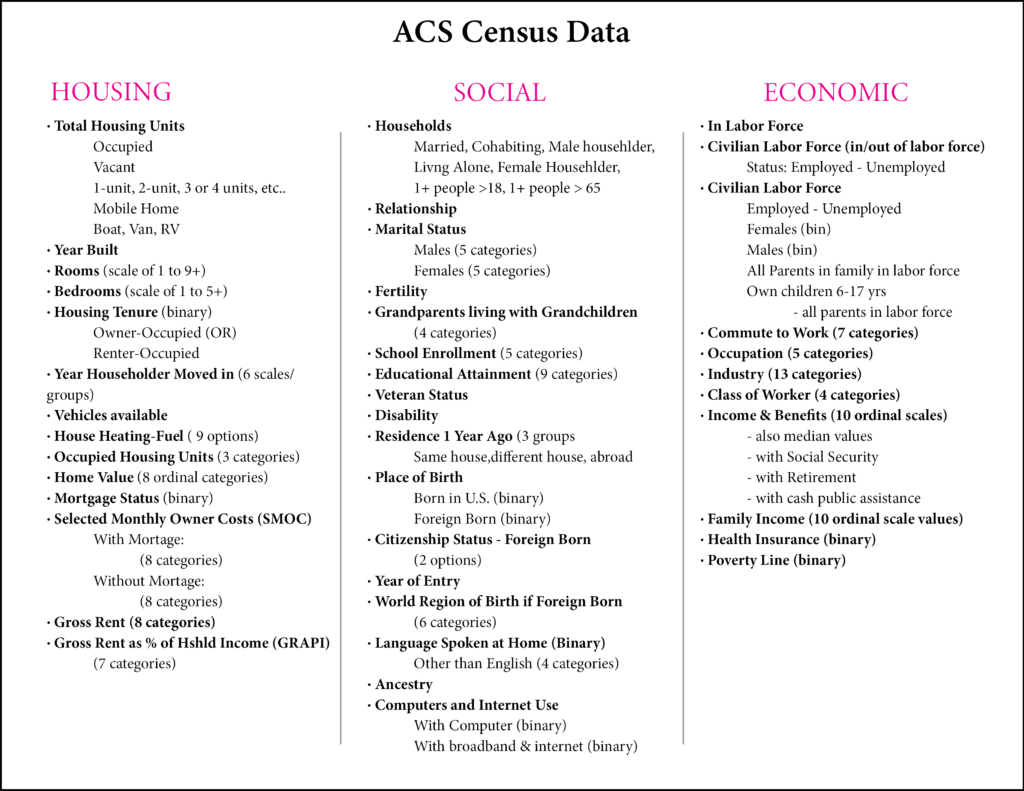
1.) The American Community Survey:
https://www.census.gov/programs-surveys/acs
All Possible Criteria:
Selected Criteria for Study:
2.) Washoe County Building Permits, 2020-2022:
A request for building permit data was filed at the Washoe County Administrative Office. While no data file or spreadsheet was procured, a secretary helped to access a building permit database, located at the following website: OneNV.us
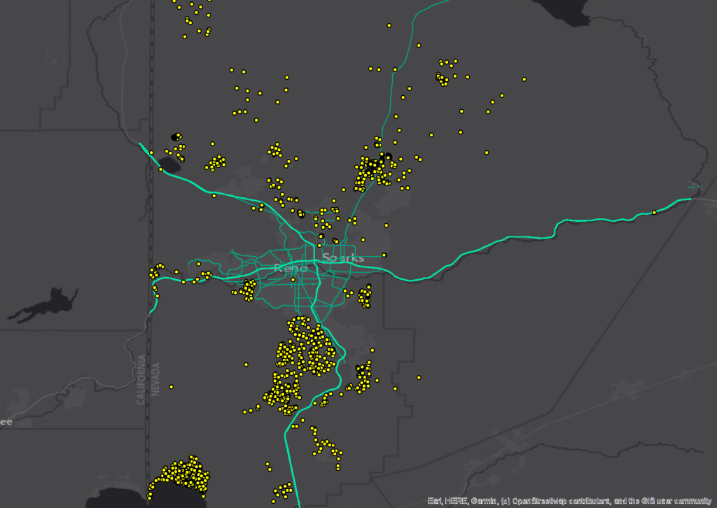
A list of over 2,000 building permits was obtained for Washoe County, dating from January 1st, 2020 to December 31st, 2021.
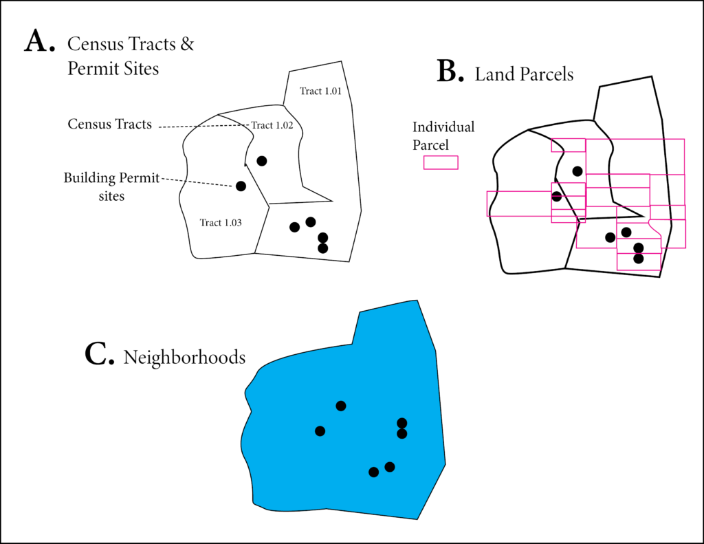
Understanding permit sites, census tracts, and land parcels.
Washoe County building permit sites, n = 2,172
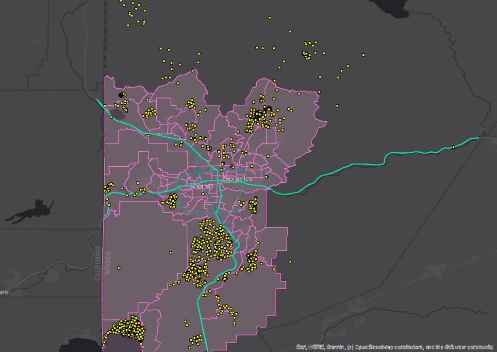
Building permit sites and census tract boundaries:
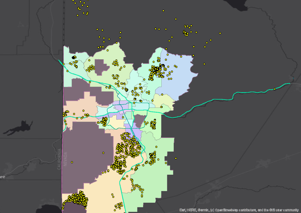
Building permit sites and neighborhoods of Reno-Sparks:
V. DATA ANALYSIS
Initial CFA results will be compared with a model that accounts for grouping at the neighborhood-level. Results from both models can be cross examined with other cities comparable to Reno-Sparks in population size.
KEY CRITERIA FOR ANALYSIS:
- Correlation Matrix for all U.S. Census data:
- Check descriptive statistics: mean, skewness, etc.
- Check fit statistics: p-values for Chi-square (low), CFI >0.8, TLI > 0.8
- Check factor loadings for all latent variables – we want the shared variance for each indicator to show to be: > 0.4, indicating a similar relationship between the chosen indicators.
- Check regression coefficients:
- View residual terms – check the covariance matrix of residual terms. Look for high outliers that may indicate a poor model, a poor latent variable
- Other Error Terms: RMSEA, SRMR
VI. BASIC DISCUSSION
Limitations are that only 105 census tracts are used for a sample size. This is below the suggested minimum of 200. Although the building permit site data is robust (over 2,000 samples), a better study would encompass more census tracts.
Another limitation is that building growth can be seen as a type of ‘blind growth’, where construction projects are resurrected with little care or importance to its surroundings or neighborhood type. Building growth is also directly related to amount of space, so ‘growth’ cannot be falsely associated with ‘prosperity’.
An key indicator that wasn’t included is the value of the buildings being constructed.
Altogether, this study will serves as a good preliminary research effort, and henceforth all data points will need to have much better granularity. For example, a neighborhood that is already densely built could be analyzed in other growth terms, like # of new business owners, or number of new bike paths, etc, and etc.
Published August 31, 2022By bargman
Categorized as Case Studies, Geography, Uncategorized Tagged Building, City Growth, Structural Equation Modeling
Leave a Reply